You are given an n x n 2D matrix representing an image, rotate the image by 90 degrees (clockwise).
You have to rotate the image in-place, which means you have to modify the input 2D matrix directly. DO NOT allocate another 2D matrix and do the rotation.
Example 1:

Input: matrix = [
    [1,2,3],
    [4,5,6],
    [7,8,9]
]

Output: [
    [7,4,1],
    [8,5,2],
    [9,6,3]
]
Example 2:

Input: matrix = [
    [5,1,9,11],
    [2,4,8,10],
    [13,3,6,7],
    [15,14,12,16]
]

Output: [
    [15,13,2,5],
    [14,3,4,1],
    [12,6,8,9],
    [16,7,10,11]
]
Example 3:

Input: matrix = [
    [1,2],
    [3,4]
]

Output: [
    [3,1],
    [4,2]
]To rotate the matrix by 90 degrees clockwise in-place, we can use a layer-by-layer rotation approach. This involves rotating the matrix in layers, starting from the outermost layer and moving inward.
-
In-Place Rotation: The problem requires modifying the matrix in-place, so we cannot use extra space for another matrix. This approach ensures that we only use constant extra space.
-
Efficient and Intuitive: By rotating the matrix layer by layer, we can systematically handle each element without complex calculations.
-
Scalable: This approach works efficiently for matrices of any size
n x n.
-
Step 1: Understand the Layers
- For an
n x nmatrix, there aren//2layers. For example: - A
3x3matrix has 1 layer. - A
4x4matrix has 2 layers.
- For an
-
Step 2: Rotate Each Layer
- For each layer, perform a four-way swap of elements:
- Move the top-left element to the top-right position.
- Move the top-right element to the bottom-right position.
- Move the bottom-right element to the bottom-left position.
- Move the bottom-left element to the top-left position.
-
Step 3: Implement the Rotation
- Use two pointers,
l(left) andr(right), to track the boundaries of the current layer. - For each layer, iterate through the elements and perform the four-way swap.
- Use two pointers,
Let’s walk through Example 1 step by step:
-
Input:
matrix = [[1,2,3],[4,5,6],[7,8,9]] -
Initialize:
l = 0,r = 2(since the matrix is3x3).
-
Rotate the Outer Layer:
- First Iteration (
i = 0):- Save the top-left element:
topLeft = matrix[0][0] = 1. - Move bottom-left to top-left:
matrix[0][0] = matrix[2][0] = 7. - Move bottom-right to bottom-left:
matrix[2][0] = matrix[2][2] = 9. - Move top-right to bottom-right:
matrix[2][2] = matrix[0][2] = 3. - Move saved top-left to top-right:
matrix[0][2] = topLeft = 1. - Updated matrix:
[7,2,1],
[4,5,6],
[9,8,3]
- Save the top-left element:
- Second Iteration (
i = 1):- Save the top-middle element:
topLeft = matrix[0][1] = 2. - Move bottom-middle to top-middle:
matrix[0][1] = matrix[1][0] = 4. - Move bottom-right-middle to bottom-middle:
matrix[1][0] = matrix[2][1] = 8. - Move top-right-middle to bottom-right-middle:
matrix[2][1] = matrix[1][2] = 6. - Move saved top-middle to top-right-middle:
matrix[1][2] = topLeft = 2. - Updated matrix:
[7,4,1],
[8,5,2],
[9,6,3]
- Save the top-middle element:
- First Iteration (
-
Result:
- The matrix is now rotated 90 degrees clockwise.
-
Output:
[[7,4,1],[8,5,2],[9,6,3]]
-
Time Complexity
-
Outer Loop: The outer loop runs for
n//2layers. -
Inner Loop: For each layer, the inner loop runs for
n - 2*layerelements. -
Overall Time Complexity:
$O(n^2)$ , wherenis the size of the matrix.
-
Outer Loop: The outer loop runs for
-
Space Complexity
- In-Place Modification: The algorithm uses only constant extra space.
-
Overall Space Complexity:
O(1).
- In-Place Rotation: The algorithm modifies the matrix in-place, satisfying the problem's constraints.
- Layer-by-Layer Rotation: By rotating the matrix layer by layer, the solution is intuitive and easy to implement.
-
Optimal Time Complexity: The time complexity of
$O(n^2)$ is optimal for this problem since we must touch every element of the matrix.
Given an m x n matrix, return all elements of the matrix in spiral order.
Example 1:

Input: matrix = [[1,2,3],[4,5,6],[7,8,9]]
Output: [1,2,3,6,9,8,7,4,5]
Example 2:

Input: matrix = [[1,2,3,4],[5,6,7,8],[9,10,11,12]]
Output: [1,2,3,4,8,12,11,10,9,5,6,7]To solve this problem, we can use a layer-by-layer traversal approach. This involves traversing the matrix in layers, starting from the outermost layer and moving inward. For each layer, we traverse the top row, right column, bottom row, and left column in order.
- Intuitive and Systematic: The layer-by-layer approach ensures that we cover all elements of the matrix in a systematic and intuitive manner.
- Efficient: This approach avoids unnecessary computations and ensures that each element is visited exactly once.
- Scalable: The solution works efficiently for matrices of any size
m x n.
-
Step 1: Define Boundaries
- Use four boundaries to represent the current layer:
left: Leftmost column of the current layer.right: Rightmost column of the current layer.top: Topmost row of the current layer.bottom: Bottommost row of the current layer.
-
Step 2: Traverse the Matrix in Spiral Order
- While
left < rightandtop < bottom:- Traverse the top row: Move from
lefttorightand add elements to the result. - Traverse the right column: Move from
top + 1tobottomand add elements to the result. - Traverse the bottom row: If
top < bottom, move fromright - 1toleftand add elements to the result. - Traverse the left column: If
left < right, move frombottom - 1totop + 1and add elements to the result.
- Traverse the top row: Move from
- After traversing a layer, update the boundaries to move to the next inner layer.
- While
-
Step 3: Handle Edge Cases
- If the matrix has only one row or one column, ensure that the traversal does not revisit elements.
Let’s walk through Example 1 step by step:
-
Input:
matrix = [[1,2,3],[4,5,6],[7,8,9]] -
Initialize Boundaries:
left = 0,right = 3(number of columns).top = 0,bottom = 3(number of rows).res = [](to store the result).
-
First Layer:
- Traverse the top row:
- Add elements from
matrix[0][0]tomatrix[0][2]:[1, 2, 3]. - Update
res = [1, 2, 3]. - Increment
topto1.
- Add elements from
- Traverse the right column:
- Add elements from
matrix[1][2]tomatrix[2][2]:[6, 9]. - Update
res = [1, 2, 3, 6, 9]. - Decrement
rightto2.
- Add elements from
- Traverse the bottom row:
- Add elements from
matrix[2][1]tomatrix[2][0]:[8, 7]. - Update
res = [1, 2, 3, 6, 9, 8, 7]. - Decrement
bottomto2.
- Add elements from
- Traverse the left column:
- Add element
matrix[1][0]:[4]. - Update
res = [1, 2, 3, 6, 9, 8, 7, 4]. - Increment
leftto1.
- Add element
- Traverse the top row:
-
Second Layer:
- Traverse the top row:
- Add element
matrix[1][1]:[5]. - Update
res = [1, 2, 3, 6, 9, 8, 7, 4, 5]. - Increment
topto2.
- Add element
- Traverse the right column:
- No elements to add (since
top == bottom).
- No elements to add (since
- Traverse the bottom row:
- No elements to add (since
left == right).
- No elements to add (since
- Traverse the left column:
- No elements to add (since
top == bottom).
- No elements to add (since
- Traverse the top row:
-
Result:
- The spiral order traversal is
[1, 2, 3, 6, 9, 8, 7, 4, 5].
- The spiral order traversal is
-
Output:
[1, 2, 3, 6, 9, 8, 7, 4, 5]
- Traversal: Each element of the matrix is visited exactly once.
- Overall Time Complexity:
O(m * n), wheremis the number of rows andnis the number of columns.
- We use an additional list
resto store the output. - The worst-case space usage is
O(m × n)(for the output). - No extra data structures are used, so
O(1)auxiliary space.
- Optimal Traversal: Each element is visited exactly once, ensuring optimal time complexity.
- In-Place Boundaries: The boundaries are updated in-place, avoiding the need for extra data structures.
- Scalable: The solution works efficiently for matrices of any size.
Given an m x n integer matrix matrix, if an element is 0, set its entire row and column to 0's.
You must do it in place.Example 1:
Example 1:
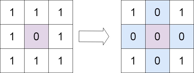
Input: matrix = [[1,1,1],[1,0,1],[1,1,1]]
Output: [[1,0,1],[0,0,0],[1,0,1]]
Example 2:
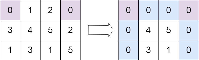
Input: matrix = [[0,1,2,0],[3,4,5,2],[1,3,1,5]]
Output: [[0,0,0,0],[0,4,5,0],[0,3,1,0]]-
Intuition
-
A brute-force approach would involve creating a separate boolean matrix to record rows and columns that should be zeroed. However, that would require O(m + n) space, violating the in-place constraint.
-
To optimize the space complexity, we use the first row and first column of the matrix itself as markers for which rows and columns should be zeroed. An additional boolean flag
rowZerotracks whether the first row needs to be zeroed.
-
- In-Place: Meets the in-place requirement by using matrix itself to track zeros.
- O(1) Space: No extra space proportional to matrix size.
- Efficient: Each element is visited at most twice.
- Avoids Redundancy: No repeated overwrites after marking.
-
Step 1: Traverse the matrix
- If
matrix[r][c] == 0, markmatrix[0][c] = 0andmatrix[r][0] = 0. - Additionally, if
r == 0, set a flagrowZero = True.
- If
-
Step 2: Zero-out the matrix (excluding first row and column)
- For
r in 1...rows-1andc in 1...cols-1, setmatrix[r][c] = 0ifmatrix[0][c] == 0ormatrix[r][0] == 0.
- For
-
Step 3: Handle first column
- If
matrix[0][0] == 0, set the first column to 0.
- If
-
Step 4: Handle first row
- If
rowZeroisTrue, set the first row to 0.
- If
-
Example for walkthrough:
matrix = [
   [0, 1, 2, 0],
   [3, 4, 5, 2],
   [1, 3, 1, 5]
]
-
Step 1: Initial Matrix
Initial:
[0, 1, 2, 0]
[3, 4, 5, 2]
[1, 3, 1, 5]
Start
rowZero = False -
Step 2: First pass to mark rows and columns
Loop through the matrix:
matrix[0][0] == 0→ markmatrix[0][0] = 0and setrowZero = Truematrix[0][3] == 0→ markmatrix[0][3] = 0- No other zeros in the matrix
Matrix now looks like:
Markers: [0, 1, 2, 0] [3, 4, 5, 2] [1, 3, 1, 5] -
Step 3: Set elements to zero based on markers
Loop through
(r=1 to 2)and(c=1 to 3):- r=1, c=1: No change
- r=1, c=2: No change
- r=1, c=3: Since
matrix[0][3] == 0, setmatrix[1][3] = 0 - r=2, c=3:
matrix[2][3] = 0
Matrix now:
After marking elements: [0, 1, 2, 0] [3, 4, 5, 0] [1, 3, 1, 0] -
Step 4: Handle first column
Since
matrix[0][0] == 0, we set:matrix[0][0] = 0matrix[1][0] = 0matrix[2][0] = 0
Matrix now:
After first column: [0, 1, 2, 0] [0, 4, 5, 0] [0, 3, 1, 0] -
Step 5: Handle first row
Since
rowZero == True, set:matrix[0][0] = 0matrix[0][1] = 0matrix[0][2] = 0matrix[0][3] = 0
Final Matrix:
[0, 0, 0, 0] [0, 4, 5, 0] [0, 3, 1, 0] -
Final Output:
[[0, 0, 0, 0], [0, 4, 5, 0], [0, 3, 1, 0]]
| Metric | Complexity | Explanation |
|---|---|---|
| Time Complexity | O(m * n) |
Each cell is visited once for marking, once for setting. |
| Space Complexity | O(1) |
No extra space used except for a few variables. |
- No Extra Matrix: We don’t use auxiliary space like a duplicate matrix or extra rows/columns.
- Constant Space: We reuse the matrix's first row and column for marking, achieving
O(1)space. - Minimized Overwrites: Logical and clean separation of marking and applying zeros avoids repeated writes.
- Scalable: Efficient even for large matrices.