ML_MATH.md

ML Math & Hands-On Intro

Linear Regression — Intuition, Math, and Visualization

---

1. Why Learn Linear Regression?

Linear Regression is usually the first Machine Learning algorithm because:

• It is simple
• It explains the core idea of ML:
  👉 Learn a pattern from data
• It introduces:
  • Model
  • Loss function
  • Optimization
  • Prediction

Almost everything in ML builds on this idea.

---

2. Real-World Intuition

Imagine you want to predict house prices.

You notice:

• Bigger houses → Higher price
• Smaller houses → Lower price

You want a straight line that best fits the data.

That line helps answer:

“If the house size is 1200 sq.ft, what should the price be?”

---

3. The Linear Regression Model

The equation of a straight line:

y = mx + b

In ML terms:

y = w·x + b

Where:

• x → input (feature)
• y → output (prediction)
• w → weight (slope)
• b → bias (intercept)

---

4. What Does the Model Really Do?

• w controls how steep the line is
• b controls where the line starts

The goal of training:

Find the best w and b so the line fits the data well.

---

5. Visualization: Data + Line

::contentReference[oaicite:0]{index=0}

• Dots → real data
• Line → model prediction
• The closer the line is to all points → better model

---

6. Prediction Example

Suppose:

w = 50
b = 10

For:

x = 20

Prediction:

y = 50 × 20 + 10 = 1010

This is how the model makes predictions.

---

7. Error (How Wrong Are We?)

Prediction is never perfect.

Error for one data point:

error = predicted_y − actual_y

Example:

actual_y = 950
predicted_y = 1010

error = 60

But errors can be positive or negative, so we square them.

---

8. Loss Function (Mean Squared Error)

Mean Squared Error (MSE):

MSE = (1/n) Σ (y_pred − y_actual)²

Why square?

• Removes negative sign
• Penalizes large mistakes

---

9. Goal of Training

Training means:

Adjust w and b
so that MSE is minimum

This is the core idea of Machine Learning.

---

10. How Do We Find Best w and b?

Intuition:

• Start with random values
• Measure loss
• Adjust slightly
• Repeat

This process is called Gradient Descent.

---

11. Gradient Descent (Conceptual)

::contentReference[oaicite:1]{index=1}

Imagine a valley:

• Top → High loss
• Bottom → Minimum loss

Gradient Descent is like:

Taking small steps downhill until you reach the bottom.

---

12. Hands-On: Simple Python Example

Step 1: Sample Data

import numpy as np

# house size
X = np.array([500, 800, 1000, 1200, 1500])
# price
y = np.array([50, 80, 100, 120, 150])

---

Step 2: Model Parameters

w = 0.0
b = 0.0
learning_rate = 0.0001

---

Step 3: Training Loop

for epoch in range(1000):
    y_pred = w * X + b
    error = y_pred - y
    
    dw = (2/len(X)) * np.sum(error * X)
    db = (2/len(X)) * np.sum(error)
    
    w -= learning_rate * dw
    b -= learning_rate * db

---

Step 4: Prediction

house_size = 1300
predicted_price = w * house_size + b
print(predicted_price)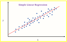

---

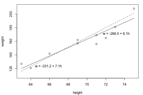
13. Visualizing the Result

• Before training → random line
• After training → best-fit line

---

14. Key Takeaways

• Linear Regression learns a straight line

• It uses:

  • Model: y = wx + b
  • Loss: Mean Squared Error
  • Optimization: Gradient Descent

• Training = minimizing error

---

15. Mental Model to Remember

Machine Learning = Guess → Measure Error → Improve Guess → Repeat

---

16. What’s Next?

After Linear Regression:

• Multiple Linear Regression
• Polynomial Regression
• Logistic Regression
• Neural Networks (same idea, more layers)

---

You now understand the math + intuition + code behind Linear Regression.