batss Python package

The batss package (batched stochastic simulator) simulates stochastic chemical reaction networks (CRNs). The package and further example notebooks can be found on Github.

If you find batss useful in a scientific project, please cite its associated paper:

Exactly simulating stochastic chemical reaction networks in sub-constant time per reaction.
Joshua Petrack and David Doty.
preprint
[ paper | BibTeX ]

Most stochastic CRN simulators use the Gillespie algorithm, which simulates one reaction at a time, so the work needed to simulate a fixed span of time grows linearly with the population size $n$. batss instead uses a batching algorithm — inspired by a batching algorithm for population protocols and adapted to general CRNs — that samples many reactions at once, taking sub-constant time per reaction. This makes large populations (billions of molecules, and beyond) practical. It falls back to Gillespie whenever that would be faster, so it is never much slower.

Crucially, batching is exact, not an approximation: it samples from precisely the same distribution as the Gillespie algorithm, unlike approximate methods such as tau-leaping.

The package is designed to be used in a Python notebook, to concisely describe a CRN, efficiently simulate its dynamics, and help visualize the result. This notebook is the source of README.md — you can download it and run every example below.

Table of contents

• Installation
• Describing a CRN
• Simulating
• Plotting the history
• Larger populations
• Running until a condition
• Long runs and log-spaced sampling
• Visualizing a single configuration
• Live visualization
• Sampling the distribution
• Time units
• More examples

Installation

The package can be installed with pip via

pip install batss

Describing a CRN

We will use the Lotka-Volterra predator-prey oscillator as a running example: rabbits $R$ breed, foxes $F$ eat rabbits and breed, and foxes starve.

$$\begin{aligned} R &\to 2R,\\ R + F &\to 2F,\\ F &\to \emptyset. \end{aligned}$$

Start by declaring the species. species takes a whitespace-separated string of names and returns one object per name.

from batss import species, Simulation

r, f = species('R F')

batss overloads Python's operators so that a reaction looks like a reaction: >> separates reactants from products, + combines species, 2*r gives a stoichiometric coefficient, and None on the product side means the reaction has no products ($\emptyset$).

rxns = [
    r >> 2*r,
    r + f >> 2*f,
    f >> None,
]

for rxn in rxns:
    print(rxn)

R -->(1.0) R + R
R + F -->(1.0) F + F
F -->(1.0) 

Rate constants default to 1. .k(...) sets the rate constant, | makes a reaction reversible, and .r(...) sets the reverse rate constant. These chain, so the reversible reaction $A + B \underset{4}{\overset{0.5}{\rightleftharpoons}} 2C$ is written as follows. (This one is just an illustration; we go back to Lotka-Volterra below.)

a, b, c = species('A B C')

print((a + b | 2*c).k(0.5).r(4))

A + B (4)<-->(0.5) C + C

Simulating

Simulation is the central object: it parses the reactions, runs the simulation, and holds the resulting data. It takes a dict of initial molecular counts, plus the reactions.

Rate constants use the standard mass-action convention, so a reaction with $k$ reactants has its rate constant divided by volume ** (k-1). By default volume is the total initial count $n$, which is usually what you want: it keeps the time scale independent of the population size, so the same reactions oscillate at the same rate whether you simulate $10^4$ molecules or $10^{10}$. (Pass volume=... explicitly if the initial counts should not define the volume.)

Let's start with ten million molecules, split evenly between rabbits and foxes.

n = 10 ** 7
sim = Simulation({r: n // 2, f: n - n // 2}, rxns, seed=0)
sim.run(10.0, 0.01)

That simulated 10 units of continuous time, recording the configuration every 0.01 time units. It is worth appreciating what just happened: with $n = 10^7$ molecules reacting for 10 time units, that is on the order of $10^8$ individual reactions, simulated exactly, in a couple of seconds.

Every recorded configuration lives in sim.history, a pandas DataFrame indexed by time.

sim.history

	F	R
time (continuous units)
0.00	5000000	5000000
0.01	4975459	5025151
0.02	4950955	5050925
0.03	4926732	5076241
0.04	4902822	5102570
...	...	...
9.96	16478249	18501490
9.97	16617193	18381164
9.98	16757114	18257799
9.99	16894304	18134443
10.00	17030406	18008948

1001 rows × 2 columns

print(sim.reactions) shows the reactions back, which is a quick way to check that batss parsed them the way you intended.

print(sim.reactions)

R -->(1.0) R + R
R + F -->(1.0) F + F
F -->(1.0) 

Plotting the history

Because history is an ordinary DataFrame, all of pandas' plotting works directly on it.

p = sim.history.plot()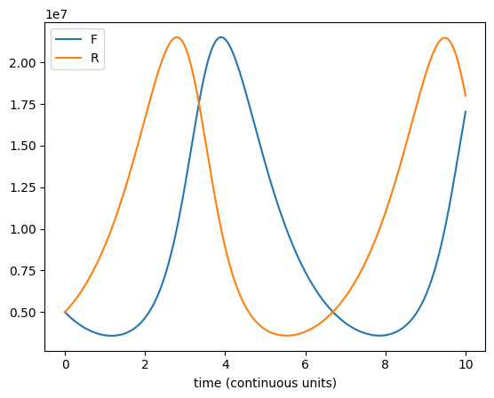

The two populations chase each other around a cycle: rabbits boom, foxes eat well and boom in turn, the rabbits crash, and then the foxes starve.

That structure is clearer in the phase plane, plotting the two counts against each other rather than against time. The deterministic Lotka-Volterra ODE has closed orbits, which would give an exactly repeating loop; the stochastic CRN instead spirals slowly outward, and it is this outward drift that eventually drives a species extinct (we come back to that below).

ax = sim.history.plot(x='R', y='F', legend=False)
ax.set_xlabel('rabbits $R$')
ax.set_ylabel('foxes $F$')
p = ax.set_title('phase plane')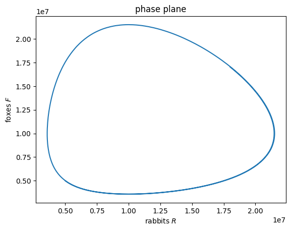

Larger populations

Batching exists so that this stays fast as $n$ grows. Here is the very same CRN with one billion molecules — around $10^{10}$ individual reactions, which a Gillespie simulator would have to step through one at a time.

n = 10 ** 9
big = Simulation({r: n // 2, f: n - n // 2}, rxns, seed=0)
big.run(10.0, 0.02)
p = big.history.plot()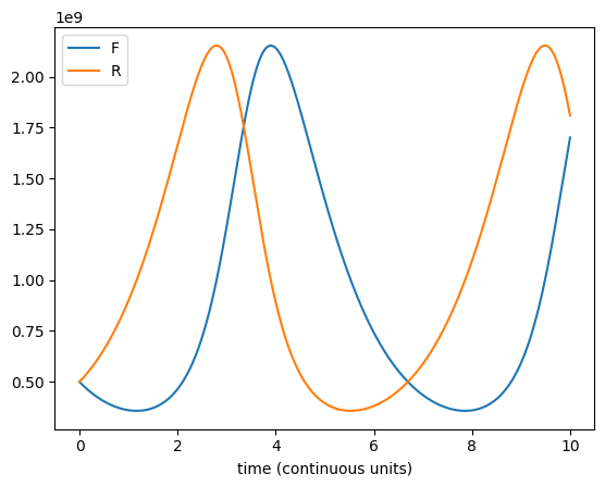

The trajectory is visibly smoother than at $n = 10^7$. Stochastic fluctuations scale like $\sqrt{n}$ while the counts themselves scale like $n$, so the relative noise shrinks as $\sqrt{1/n}$ and the CRN behaves more and more like its deterministic limit.

Running until a condition

Instead of a fixed end time, run_until accepts a convergence detector: any function taking the current configuration (a dict mapping species to counts) and returning a bool. The simulation runs until it returns True.

Lotka-Volterra is a nice example, because the stochastic model does something the deterministic one never does. The ODE cycles forever, but at any finite $n$ the outward spiral we saw above eventually overshoots, one species undershoots to zero, and it is gone for good.

def one_species_extinct(config):
    return config.get(r, 0) == 0 or config.get(f, 0) == 0


n = 1000
small = Simulation({r: n // 2, f: n - n // 2}, rxns, seed=0)
small.run(one_species_extinct, 0.05)

print(f'extinction at time {small.time:.0f}')
print(small.config_dict)

extinction at time 1154
{R: 50}

A word of warning. Calling run() with no arguments runs until the configuration is silent, meaning no reaction can occur at all. For Lotka-Volterra that is not safe: if the foxes die out first, then nothing stops $R \to 2R$, the rabbits breed without bound, and the configuration is never silent — so run() would never return. Use a convergence detector whenever silence is not guaranteed.

The extinction itself is invisible on a linear axis: the counts fall through several orders of magnitude in the last few oscillations, and everything below a few hundred is squashed onto the $x$-axis. Matplotlib's symlog scale (linear near zero, logarithmic above it) shows the whole descent. Here are the last 120 time units, where the oscillations grow until one species finally undershoots to zero.

endgame = small.history.loc[small.time - 120:]

ax = endgame.plot()
ax.set_yscale('symlog')
ax.set_ylim(bottom=0)   # symlog would otherwise show a meaningless negative range
p = ax.set_title('the last 120 time units before extinction')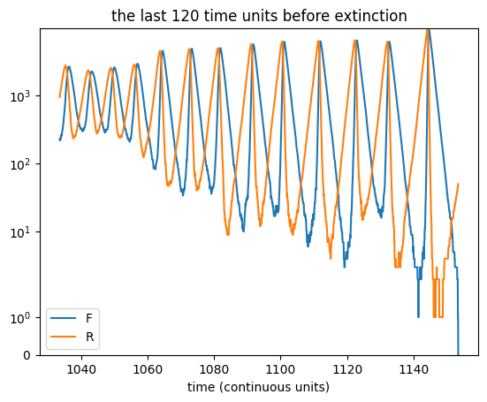

Long runs and log-spaced sampling

We did not know in advance how long that run would take, and with a fixed history_interval a long run records a great many nearly identical configurations. history_interval may instead be a function of the current time, so that recording gets steadily coarser as the simulation goes on — keeping the history to a manageable size without losing detail early on, when things are changing fastest.

coarse = Simulation({r: n // 2, f: n - n // 2}, rxns, seed=0)
coarse.run(one_species_extinct, history_interval=lambda t: max(0.05, t / 200))

print(f'{len(coarse.history)} configurations recorded, '
      f'vs {len(small.history)} for the fixed interval above')

902 configurations recorded, vs 23071 for the fixed interval above

Visualizing a single configuration

Each row of sim.history is one configuration, so a single row can be drawn as a barplot. Here is the $n = 10^7$ simulation at two different times.

from matplotlib import pyplot as plt


def plot_row(row):
    fig, ax = plt.subplots(figsize=(4, 3))
    sim.history.iloc[row].plot(
        ax=ax, kind='bar', ylim=(0, sim.n), rot=0, xlabel='species', ylabel='count',
        title=f'Lotka-Volterra at time {sim.history.index[row]:.2f}')


plot_row(0)
plot_row(300)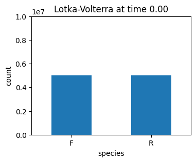

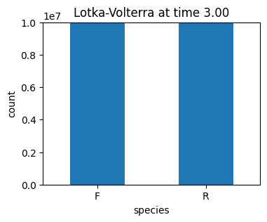
ipywidgets turns that into a slider that scrubs through the whole history.

import ipywidgets as widgets

bar = widgets.interact(plot_row, row=widgets.IntSlider(
    min=0, max=len(sim.history) - 1, step=1, value=0, layout=widgets.Layout(width='100%')))

Dragging that slider walks the barplot through the whole simulation, and the two species visibly take turns:

Live visualization

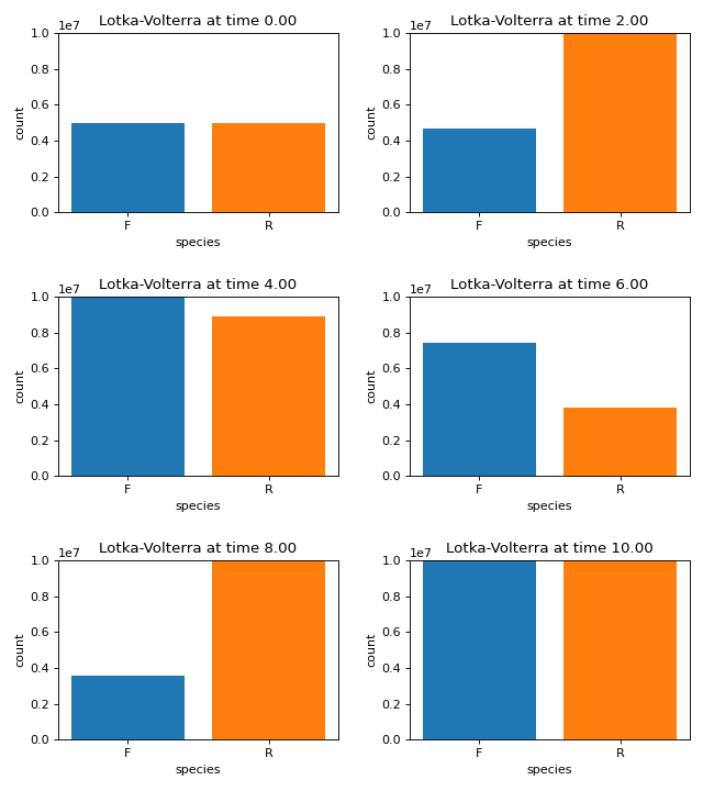
Everything above plots after the simulation finishes. A Snapshot plots while it runs: StatePlotter is a barplot of the current configuration and HistoryPlotter is a line plot of the history so far. sim.add_snapshot(...) attaches one, and it then redraws periodically during run.

To actually watch these update live, you need an interactive matplotlib backend: pip install ipympl, then put %matplotlib widget at the top of the notebook. Jupyter Lab is the recommended environment; unfortunately Google Colab does not support these backends. With the default inline backend, as here, the figure simply shows the final state of the run.

from batss.snapshot import StatePlotter

n = 10 ** 5
live = Simulation({r: n // 2, f: n - n // 2}, rxns, seed=1)
live.add_snapshot(StatePlotter())
live.run(20.0, 0.1)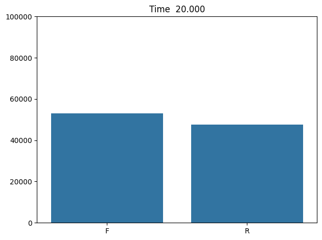

Once the run is done, snapshot_slider gives back a slider that moves every attached snapshot backwards and forwards through the recorded history.

live.snapshot_slider('time')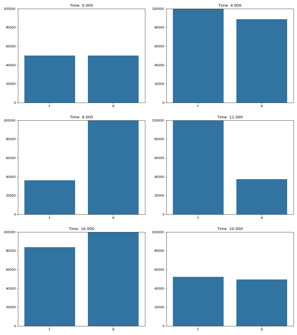

The difference between this and the previous slider is who is doing the work: there we wrote plot_row and wired up ipywidgets ourselves, whereas here batss redraws every Snapshot attached to the simulation, so one slider drives them all.

Sampling the distribution

A single run is just one sample from the CRN's distribution. sample_future_configuration restarts from the current configuration many times over, and returns a DataFrame whose rows are the independent trials — exactly the shape a histogram wants.

n = 10 ** 5
dist = Simulation({r: n // 2, f: n - n // 2}, rxns, seed=1)
samples = dist.sample_future_configuration(5.0, num_samples=500)
samples.describe().loc[['mean', 'std', 'min', 'max']]

	F	R
mean	139688.268000	39505.234000
std	1015.495328	637.814165
min	136911.000000	37642.000000
max	141977.000000	41401.000000

p = samples.plot(kind='hist', bins=40, alpha=0.6,
                 title='distribution of counts at time 5, over 500 trials')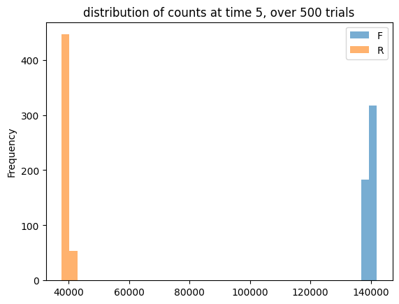

Time units

Rate constants usually come with physical units attached. time_units — any string that pandas.to_timedelta accepts, such as 'seconds' — makes the history index a pandas TimedeltaIndex rather than a plain float index, so the history carries real units and pandas' time series machinery (resampling, and so on) applies to it.

n = 10 ** 5
timed = Simulation({r: n // 2, f: n - n // 2}, rxns, time_units='seconds', seed=1)
timed.run(20.0, 0.05)

timed.history.index[:3]

TimedeltaIndex(['0 days 00:00:00', '0 days 00:00:00.050000',
                '0 days 00:00:00.100000'],
               dtype='timedelta64[ns]', freq=None)

One wrinkle worth knowing about. A pandas Timedelta is a duration, and it always prints in the form [D days ]HH:MM:SS.fff — there is no way to ask it to render itself as a plain number of seconds. So the tick at two and a half seconds is labelled 00:00:02.5, not 2.5, and those ten-character labels are wide enough to collide with each other. Rotating them fixes it (batss's own HistoryPlotter does the same thing whenever time_units is set).

ax = timed.history.plot()
p = ax.tick_params(axis='x', rotation=45)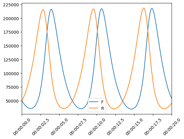

More examples

• examples/crn_examples.ipynb — the same tools applied to four more CRNs: dimerization, the Rössler-Willamowski attractor, the Oregonator, and the Brusselator.
• benchmark/benchmark.ipynb — how batss's running time scales with the population size, measured against the Gillespie algorithm.
• API documentation