quarto.qmd

# Quarto {#sec-quarto}

In this chapter, you'll get more in-depth with [**Quarto**](https://quarto.org/), following a brief introduction in @sec-workflow-writing-code. **Quarto** is a tool that allows you to combine code and text (in the form of markdown, covered in @sec-markdown) and create rich outputs, like reports and presentations.

## Introduction

Quarto is a unified authoring framework for data science, combining your code, its results, and your prose commentary. Quarto allows for outputs that are fully reproducible and it supports dozens of output formats, like PDFs, Microsoft Word files, slideshows, and more.

Quarto markdown is designed to be used in three ways:

1. For communicating to decision makers, who want to focus on the conclusions, not the code behind the analysis.

2. For collaborating with other data scientists (including future you!), who are interested in both your conclusions, and how you reached them (i.e. the code).

3. As an environment in which to *do* data science, as a modern day lab notebook where you can capture not only what you did, but also what you were thinking.

For example, a use case would be a technical report exploring recent trade statistics in which the code part pulls down the latest data and plots it. Or you could do the same analysis, but push it to a website. Best of all, you can decide whether to hide or show the code parts in the final outputs (or, with html outputs, allow users to choose whether to see the code or not). In more detail, use cases include:

- reports that use data and/or charts and that are similar each time they are run (eg only the data are updated)

- technical reports that show or use the functionality of an existing code base

- slide decks that summarise the most recent data and that are produced at a regular frequency

- sending exploratory or prototype analysis to co-authors or collaborators

- writing blogs for blogging services that accept `.md` files (make sure to export to markdown)

- creating automatically updated websites relatively easily——we won’t cover that in this chapter, but you can find some information on this [here](https://quarto.org/docs/websites/).

**Quarto** is a really convenient wrapper for a bunch of other tools that makes it convenient to produce automated reports. You should check the latest [documentation](https://quarto.org/docs/getting-started/quarto-basics.html) for an up to date guide on use——here, we're going to see the basics and introduce a couple of templates that will serve you well.

### Prerequisites

You will need to go to the [**Quarto** website](https://quarto.org/) and follow the [install instructions](https://quarto.org/docs/getting-started/installation.html) first. You can check you've installed it properly using `quarto check install` on the command line.

You may also find the Visual Studio Code [quarto extension](https://marketplace.visualstudio.com/items?itemName=quarto.quarto) useful and this book recommends it. This creates a special button within Visual Studio code labelled "render" that shows you how the output will look side-by-side with the input.

## Automated Reports with **Quarto**

Quarto can be used to create *output* documents and slides in a wide variety of formats including HTML, PDF, Microsoft Office (docx and pptx), OpenOffice, and many more.

You can write the *input* documents (include code snippets) in two possible ways:

1. A special kind of markdown file, with file extension `.qmd`. For more on markdown, see @sec-markdown. Code blocks that have a special syntax get executed and their results are included in any outputs.

2. Jupyter Notebooks, with file extension `.ipynb`. Code cells are executed and their results are included in any outputs.

You optionally add code (e.g. Python, R, JavaScript, etc.) to the documents to dynamically create figures, tables, etc. and then render the documents to their final format using Quarto.

### A minimal example of a report written with markdown content

We're now going to try the most minimal example of the first approach, a `.qmd` file, that also includes code and outputs.

There are advantages and disadvantages to writing your report in the `.qmd` format. The advantage is that it's just a plain text file and therefore anyone can open it, look at it, and change it with a text editor (and it's more convenient for version control in this way too). The big, big disadvantage is that you cannot see how the code is coming on as you write it (you have to render it to see the code outputs, as we'll see in a moment). In the next sub-section, we'll see a way of achieving a better workflow.

Let's get our minimal example setup. The below code and markdown form the content of a file called `report.qmd`:

````markdown
---
title: "Example Report"
author: "Joan Robinson"
format: pdf
toc: true
number-sections: true
jupyter: python3
---

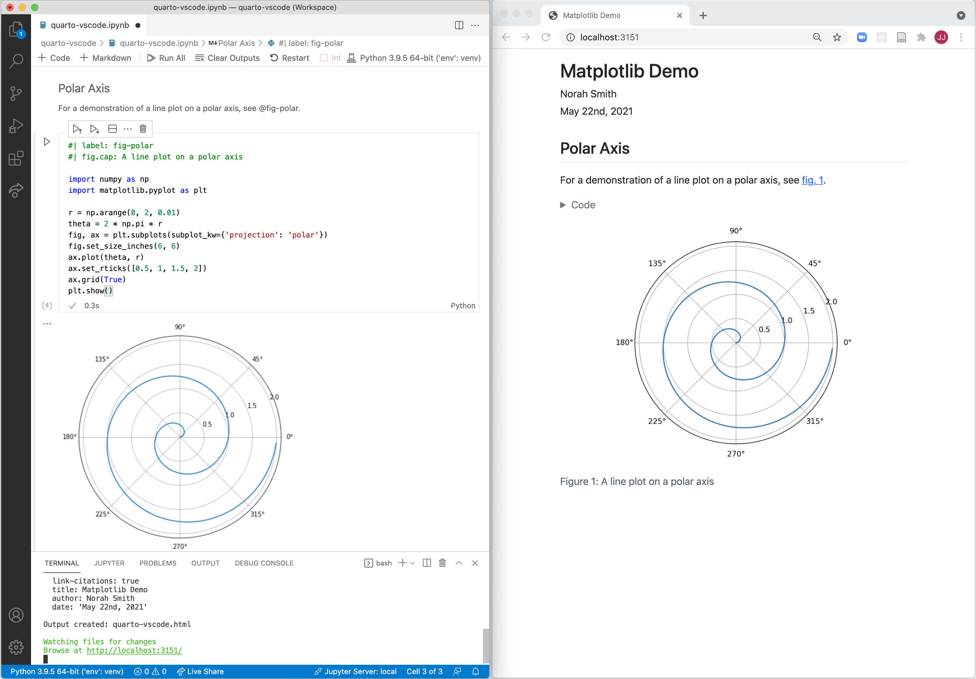
## Polar Axis

For a demonstration of a line plot on a polar axis, see @fig-polar.

```{{python}}
#| label: fig-polar
#| fig-cap: "A line plot on a polar axis"

import numpy as np
import matplotlib.pyplot as plt

r = np.arange(0, 2, 0.01)
theta = 2 * np.pi * r
fig, ax = plt.subplots(subplot_kw={'projection': 'polar'})
ax.plot(theta, r)
ax.set_rticks([0.5, 1, 1.5, 2])
ax.grid(True)
plt.show()
```
````

This example contains three important types of content:

1. A **YAML header** surrounded by `---`s.
2. **Chunks** of Python code surrounded by ```` ``` ````.
3. Markdown mixed with simple text formatting like `# heading` and `_italics_`.

In this 'raw' input quarto markdown `.qmd` file, `{python}` tells **Quarto** that a code chunk is in Python and should be executed, and `jupyter: python3` tells **Quarto** what installation of Jupyter Notebooks to use. If you're unsure what your installation of Jupyter is called, you can see a list by running `jupyter kernelspec list` on the command line.

### Rendering into Output Documents

To turn the above report into an output PDF, save it as `report.qmd` and then, on the command line and in the same directory as the file, run

```bash
quarto render report.qmd
```

Remember that if you are using the Visual Studio Code [quarto extension](https://marketplace.visualstudio.com/items?itemName=quarto.quarto) (recommended), you can hit the render button instead (but you'll need to choose PDF as the output).

::: {.callout-tip title="Exercise"}
Successfuly create a PDF by saving the markdown above into a file called `report.qmd`.

If you get an error about not being able to find the Jupyter kernel, first check you have Jupyter Lab installed and then check what your Jupyter kernel is called using `jupyter kernelspec list` on the command line. You need to specify the name of your Jupyter kernel correct in the header document (in the example above, it's called 'python3', which is the default).

:::

Now, because we specified `pdf` in the 'header' of our file we automatically got a pdf. But a wide range of output formats are available. For example, HTML

```bash
quarto render report.qmd --to html
```

and Microsoft Word

```bash
quarto render report.qmd --to docx
```

One slight frustration with the conversion to Word Documents is that tables from code (data frames) are not rendered as tables in the Word doc.

The basic syntax is to write `--to outputformat` at the end of the render command.

::: {.callout-tip title="Exercise"}
Successfully create a HTML report by saving the markdown above into a file called `report.qmd` and then running the quarto render command with the to html option.

What happens to the menu on the right-hand side as you add extra headings using the `##` markdown syntax?

:::

### Code Block Execution Options

There are different options for how the code block is executed. To include a code block that doesn't get executed, just use regular markdown syntax (ie a block that begins ```` ```python ````). Otherwise, you have rich options about whether to show the input code, just the results, both, or neither (while still executing the code). 

For an example of a code output where the input is not shown, the code below will *only* show the output table by using the `echo: false` option.

````
```{{python}}
#| echo: false
import pandas as pd
import seaborn as sns

df = sns.load_dataset("penguins")
pd.crosstab(df["species"], [df["island"], df["sex"]], margins=True)
```
````

The table below gives all of the options for code blocks.

  | Option    | Description                                                                                                                                                                                 |
  | --------- | ------------------------------------------------------------------------------------------------------------------------------------------------------------------------------------------- |
  | `eval`    | Evaluate the code chunk (if false, just echos the code into the output).                                                                                                                    |
  | `echo`    | Include the source code in output                                                                                                                                                           |
  | `output`  | Include the results of executing the code in the output (true, false, or asis to indicate that the output is raw markdown and should not have any of Quarto’s standard enclosing markdown). |
  | `warning` | Include warnings in the output.                                                                                                                                                             |
  | `error`   | Include errors in the output (note that this implies that errors executing code will not halt processing of the document).                                                                  |
  | `include` | Catch all for preventing any output (code or results) from being included (e.g. include: false suppresses all output from the code block).                                                  |
  | `true`    | True                                                                                                                                                                                        |
  | `false`   | False                                                                                                                                                                                       |

It's also **possible to insert code results in-line with text**. Here's a minimal example of that.

````markdown
---
title: "Example Report with Inline Numbers from Code"
author: "Joan Robinson"
format: pdf
toc: true
number-sections: true
jupyter: python3
---

## Report

For a demonstration of a line plot on a polar axis, see @fig-polar.

For an example of a code output where the input is not shown, the code below will *only* show the output table by using the `echo: false` option.

```{{python}}
#| echo: false
from IPython.display import display, Markdown
import pandas as pd
import seaborn as sns

df = sns.load_dataset("penguins")
big_pen = df["body_mass_g"].max()
number = len(df)
```

### The Heaviest Penguin

We find that the heaviest penguin, out of a total of `python f"{number}"` penguins, has a mass of `python f"{big_pen:.2f}"` kilograms.

````

Note that, in this example, the `:2f` part of `{big_pen:.2f}` is an instruction to report the given number to 2 decimal places.

::: {.callout-tip title="Exercise"}
Create a HTML report with an in-line number using the above example but change the formatting of the heaviest penguin to not show any decimal places.

:::

There are, of course, lots of extra features that go beyond this example.

### A minimal example of a report written with Jupyter Notebooks

You can also write your reports with Jupyter Notebooks. As a reminder, these have cells that can be either text (in the form of markdown) or code (and they support a lot of languages), and have the file format `.ipynb`. This book recommends working with them in Visual Studio Code. Google Colab notebooks are a type of Jupyter notebook (and can be downloaded as `.ipynb` files).

Writing your automated reports in Jupyter Notebooks has one major advantage over using `.qmd` markdown files: you can run the code as you go, so you know what you're getting and it's easier to weed out bugs. This book recommends this approach to writing automated reports.

So what is the difference from what we've seen above? Very little, actually. Your content will still start with exactly the same header but this time it's going to be in a *markdown cell* at the top of your notebook. To be explicit, the first cell in your notebook will have:

```markdown
---
title: "Example Report"
author: "Joan Robinson"
format: pdf
toc: true
number-sections: true
jupyter: python3
---
```

Subsequent cells will be code or markdown depending on whether you need rich outputs (figures and tables) or text. So, instead of a code chunk that begins with ```` ```{python} ```` like in the `.qmd` approach, you will just create a new code cell.

Remember that putting `format: pdf` into this header will mean that the `render` command automatically produces a pdf. You can change it to `format: html` to default to a html file instead—and both options can be over-written by passing `--to format`.

As before, you can create text that is dynamically updated with code outputs too; just choose a code cell rather than a markdown cell.

The main difference when it comes to Jupyter Notebooks is that you must decide whether you want to *execute* the notebook before you render it with **Quarto**. Executing a notebook just means run the code before exporting it to a new format. (As an aside, the best practice way to use Jupyter Notebooks is to save them without any code outputs, so execute and render would be the standard way of doing it.) The terminal command to run a notebook and render it is:

```bash
quarto render jupyter-report.ipynb --execute
```

::: {.callout-tip title="Exercise"}
Create a new Jupyter Notebook called `jupyter-report.ipynb` with the header above. Re-use the blocks of code and text from the `qmd` example in the previous section. Render it with the command above.

:::

To change the output type, add another instruction to the command using `--to`:

```bash
quarto render jupyter-report.ipynb --execute --to html
```

## The Optimal Workflow for Writing Automated Reports

This is an alternative to using the Visual Studio Code **Quarto** extension.

We now turn to a big tip on the optimal workflow for making automated reports and slides. Often you are interested in seeing how the final report will look as you change the code in *real time*. This is possible with Jupyter Notebooks and **Quarto**. Run the following in the terminal

```bash
quarto preview jupyter-report.ipynb
```

A browser window will open with a live preview of your pdf (if you set pdf as the default output option in the header). To create a live preview of a HTML document, it's

```bash
quarto preview jupyter-report.ipynb --to html
```

The image below shows an example of using preview side-by-side with a Jupyter Notebook in Visual Studio Code.

![Jupyter notebook and live HTML preview of generated report](https://quarto.org/docs/tools/images/vscode-preview.png)

::: {.callout-tip title="Exercise"}
Take the Jupyter example from the previous exercise and change the format to HTML. Then add both a new text cell and a new figure (from a code cell) while in preview mode, making use of the `quarto preview` command above. If you need inspiration for the new figure, here's a simple scatter plot:

```python
import numpy as np
import matplotlib.pyplot as plt

fig, ax = plt.subplots()
ax.scatter(
    [1, 2, 3, 4, 5, 6],
    [1, 4, 2, 3, 1, 7],
    s=np.linspace(300, 2000, 6),
    c=["b", "r", "g", "k", "cyan", "yellow"],
    edgecolors="k",
    alpha=0.5,
)
plt.show()
```

:::

## Automated Slides with **Quarto**

It isn't just reports that you can create; you can make slide decks too. You have three main output formats to choose from for slides:

- html, via something called 'revealjs'; use `format: revealjs`
- pdf, via the LaTeX beamer package; use `format: beamer`
- Powerpoint, using the pptx format; use `format: pptx`

Everything else is the same as we have seen before. Here's a minimal example showing both code and text. It creates a HTML slide deck.

````markdown
---
title: "My Talk"
author: "Joan Robinson"
format: revealjs
---

## Introduction

- This is some text
- As is this

## Here Are Some Code Outputs

```{{python}}
#| echo: false
import numpy as np
import matplotlib.pyplot as plt

r = np.arange(0, 2, 0.01)
theta = 2 * np.pi * r
fig, ax = plt.subplots(subplot_kw={'projection': 'polar'})
ax.plot(theta, r)
ax.set_rticks([0.5, 1, 1.5, 2])
ax.grid(True)
plt.show()
```
````

Note that this will not show the code, only the figure, as we have set `#| echo: false` for the code chunk. You could also set `echo: false` for the whole deck in the header.

::: {.callout-tip title="Exercise"}
Render this slide example in all three of the main formats
:::

::: {.callout-tip title="Exercise"}
Add outputs from in-line code into your rendered deck, adapting the heaviest penguin example from earlier.
:::