Interpolation.fsx

(**
---
title: Interpolation
index: 8
category: Documentation
categoryindex: 0
---
*)

(*** hide ***)

(*** condition: prepare ***)
#r "nuget: FSharpAux.Core, 2.0.0"
#r "nuget: FSharpAux, 2.0.0"
#r "nuget: FSharpAux.IO, 2.0.0"
#r "nuget: OptimizedPriorityQueue, 5.1.0"
#r "nuget: FsMath, 0.0.2"
#I "../src/FSharp.Stats/bin/Release/.net8.0/"
#r "FSharp.Stats.dll"
#r "nuget: Plotly.NET, 4.0.0"
open FsMath

Plotly.NET.Defaults.DefaultDisplayOptions <-
    Plotly.NET.DisplayOptions.init (PlotlyJSReference = Plotly.NET.PlotlyJSReference.NoReference)

(*** condition: ipynb ***)
#if IPYNB
#r "nuget: Plotly.NET, 4.0.0"
#r "nuget: Plotly.NET.Interactive, 4.0.0"
#r "nuget: FSharp.Stats"

open Plotly.NET
#endif // IPYNB

(**

# Interpolation

[![Binder](https://mybinder.org/badge_logo.svg)](https://mybinder.org/v2/gh/fslaborg/FSharp.Stats/gh-pages?urlpath=/tree/home/jovyan/Interpolation.ipynb)
[![Notebook]({{root}}img/badge-notebook.svg)]({{root}}{{fsdocs-source-basename}}.ipynb)

_Summary:_ This tutorial demonstrates several ways of interpolating with FSharp.Stats

## Summary

With the `FSharp.Stats.Interpolation` module you can apply various interpolation methods. While interpolating functions always go through the input points (knots), methods to predict function values 
from x values (or x vectors in multivariate interpolation) not contained in the input, vary greatly. A `Interpolation` type provides many common methods for interpolation of two dimensional data. These include

- Linear spline interpolation (connecting knots by straight lines)
- Polynomial interpolation
- Hermite spline interpolation
- Cubic spline interpolation with 5 boundary conditions
- Akima subspline interpolation

The following code snippet summarizes all interpolation methods. In the following sections, every method is discussed in detail!

*)

open Plotly.NET
open FSharp.Stats

let testDataX = [|1. .. 10.|]

let testDataY = [|0.5;-1.;0.;0.;0.;0.;1.;1.;3.;3.5|]

let coefStep        = Interpolation.interpolate(testDataX,testDataY,InterpolationMethod.Step) // step function
let coefLinear      = Interpolation.interpolate(testDataX,testDataY,InterpolationMethod.LinearSpline) // Straight lines passing all points
let coefAkima       = Interpolation.interpolate(testDataX,testDataY,InterpolationMethod.AkimaSubSpline) // Akima cubic subspline
let coefCubicNa     = Interpolation.interpolate(testDataX,testDataY,InterpolationMethod.CubicSpline Interpolation.CubicSpline.BoundaryCondition.Natural) // cubic spline with f'' at borders is set to 0
let coefCubicPe     = Interpolation.interpolate(testDataX,testDataY,InterpolationMethod.CubicSpline Interpolation.CubicSpline.BoundaryCondition.Periodic) // cubic spline with equal f' at borders
let coefCubicNo     = Interpolation.interpolate(testDataX,testDataY,InterpolationMethod.CubicSpline Interpolation.CubicSpline.BoundaryCondition.NotAKnot) // cubic spline with continous f''' at second and penultimate knot
let coefCubicPa     = Interpolation.interpolate(testDataX,testDataY,InterpolationMethod.CubicSpline Interpolation.CubicSpline.BoundaryCondition.Parabolic) // cubic spline with quadratic polynomial at borders
let coefCubicCl     = Interpolation.interpolate(testDataX,testDataY,InterpolationMethod.CubicSpline (Interpolation.CubicSpline.BoundaryCondition.Clamped (0,-1))) // cubic spline with border f' set to 0 and -1
let coefHermite     = Interpolation.interpolate(testDataX,testDataY,InterpolationMethod.HermiteSpline HermiteMethod.CSpline)
let coefHermiteMono = Interpolation.interpolate(testDataX,testDataY,InterpolationMethod.HermiteSpline HermiteMethod.PreserveMonotonicity)
let coefHermiteSlop = Interpolation.interpolate(testDataX,testDataY,InterpolationMethod.HermiteSpline (HermiteMethod.WithSlopes (vector [0.;0.;0.;0.;0.;0.;0.;0.;0.;0.])))
let coefPolynomial  = Interpolation.interpolate(testDataX,testDataY,InterpolationMethod.Polynomial) // interpolating polynomial 
let coefApproximate = Interpolation.Approximation.approxWithPolynomialFromValues(testDataX,testDataY,10,Interpolation.Approximation.Spacing.Chebyshev) //interpolating polynomial of degree 9 with knots spaced according to Chebysehv

let interpolationComparison =
    [
        Chart.Point(testDataX,testDataY,Name="data")
        [1. .. 0.01 .. 10.] |> List.map (fun x -> x,Interpolation.predict(coefStep)        x) |> Chart.Line |> Chart.withTraceInfo "Step"
        [1. .. 0.01 .. 10.] |> List.map (fun x -> x,Interpolation.predict(coefLinear)      x) |> Chart.Line |> Chart.withTraceInfo "Linear"
        [1. .. 0.01 .. 10.] |> List.map (fun x -> x,Interpolation.predict(coefAkima)       x) |> Chart.Line |> Chart.withTraceInfo "Akima"
        [1. .. 0.01 .. 10.] |> List.map (fun x -> x,Interpolation.predict(coefCubicNa)     x) |> Chart.Line |> Chart.withTraceInfo "Cubic_natural"
        [1. .. 0.01 .. 10.] |> List.map (fun x -> x,Interpolation.predict(coefCubicPe)     x) |> Chart.Line |> Chart.withTraceInfo "Cubic_periodic"
        [1. .. 0.01 .. 10.] |> List.map (fun x -> x,Interpolation.predict(coefCubicNo)     x) |> Chart.Line |> Chart.withTraceInfo "Cubic_notaknot"
        [1. .. 0.01 .. 10.] |> List.map (fun x -> x,Interpolation.predict(coefCubicPa)     x) |> Chart.Line |> Chart.withTraceInfo "Cubic_parabolic"
        [1. .. 0.01 .. 10.] |> List.map (fun x -> x,Interpolation.predict(coefCubicCl)     x) |> Chart.Line |> Chart.withTraceInfo "Cubic_clamped"
        [1. .. 0.01 .. 10.] |> List.map (fun x -> x,Interpolation.predict(coefHermite)     x) |> Chart.Line |> Chart.withTraceInfo "Hermite cSpline"
        [1. .. 0.01 .. 10.] |> List.map (fun x -> x,Interpolation.predict(coefHermiteMono) x) |> Chart.Line |> Chart.withTraceInfo "Hermite monotone"
        [1. .. 0.01 .. 10.] |> List.map (fun x -> x,Interpolation.predict(coefHermiteSlop) x) |> Chart.Line |> Chart.withTraceInfo "Hermite slope"
        [1. .. 0.01 .. 10.] |> List.map (fun x -> x,Interpolation.predict(coefPolynomial)  x) |> Chart.Line |> Chart.withTraceInfo "Polynomial"
        [1. .. 0.01 .. 10.] |> List.map (fun x -> x,coefApproximate.Predict x)                |> Chart.Line |> Chart.withTraceInfo "Chebyshev"
    ]
    |> Chart.combine
    |> Chart.withTemplate ChartTemplates.lightMirrored
    |> Chart.withXAxisStyle("x data")
    |> Chart.withYAxisStyle("y data")
    |> Chart.withSize(800.,600.)

(*** condition: ipynb ***)
#if IPYNB
interpolationComparison
#endif // IPYNB

(***hide***)
interpolationComparison |> GenericChart.toChartHTML
(***include-it-raw***)

(**

## Polynomial Interpolation

Here a polynomial is fitted to the data. In general, a polynomial with degree = dataPointNumber - 1 has sufficient flexibility to interpolate all data points.
The least squares approach is not sufficient to converge to an interpolating polynomial! A degree other than n-1 results in a regression polynomial.

*)


open Plotly.NET
open FSharp.Stats

let xData = vector [|1.;2.;3.;4.;5.;6.|]
let yData = vector [|4.;7.;9.;8.;7.;9.;|]

//Polynomial interpolation

//Define the polynomial coefficients. In Interpolation the order is equal to the data length - 1.
let coefficients = 
    Interpolation.Polynomial.interpolate xData yData 
let interpolFunction x = 
    Interpolation.Polynomial.predict coefficients x

let rawChart = 
    Chart.Point(xData,yData)
    |> Chart.withTraceInfo "raw data"
    
let interpolPol = 
    let fit = [|1. .. 0.1 .. 6.|] |> Array.map (fun x -> x,interpolFunction x)
    fit
    |> Chart.Line
    |> Chart.withTraceInfo "interpolating polynomial"

let chartPol = 
    [rawChart;interpolPol] 
    |> Chart.combine
    |> Chart.withTemplate ChartTemplates.lightMirrored

(*** condition: ipynb ***)
#if IPYNB
chartPol
#endif // IPYNB

(***hide***)
chartPol |> GenericChart.toChartHTML
(***include-it-raw***)

(**
## Cubic spline interpolation

Splines are flexible strips of wood, that were used by shipbuilders to draw smooth shapes. In graphics and mathematics a piecewise cubic polynomial (order = 3) is called spline.
The curvature (second derivative) of a cubic polynomial is proportional to its tense energy and in spline theory the curvature is minimized. Therefore, the resulting function is very smooth.
To solve for the spline coefficients it is necessary to define two additional constraints, so called boundary conditions:

 - natural spline (most used spline variant): `f''` at borders is set to 0

 - periodic spline: `f'` at first point is the same as `f'` at the last point

 - parabolic spline: `f''` at first/second and last/penultimate knot are equal

 - notAKnot spline: `f'''` at second and penultimate knot are continuous

 - quadratic spline: first and last polynomial are quadratic, not cubic

 - clamped spline: `f'` at first and last knot are set by user

In general, piecewise cubic splines only are defined within the region defined by the used x values. Using `predict` with x values outside this range, uses the slopes and intersects of the nearest knot and utilizes them for prediction.

### Related information
 - [Cubic Spline Interpolation](https://en.wikiversity.org/wiki/Cubic_Spline_Interpolation)

 - [Boundary conditions](https://timodenk.com/blog/cubic-spline-interpolation/)

 - [Cubic spline online tool](https://tools.timodenk.com/cubic-spline-interpolation)
*)


open Plotly.NET
open FSharp.Stats.Interpolation

let xValues = vector [1.;2.;3.;4.;5.5;6.]
let yValues = vector [1.;8.;6.;3.;7.;1.]

//calculates the spline coefficients for a natural spline
let coeffSpline = 
    CubicSpline.interpolate CubicSpline.BoundaryCondition.Natural xValues yValues

//cubic interpolating splines are only defined within the region defined in xValues
let interpolateFunctionWithinRange  x = 
    CubicSpline.predictWithinRange coeffSpline x

//to interpolate x_Values that are out of the region defined in xValues
//interpolates the interpolation spline with linear prediction at borderknots
let interpolateFunction x = 
    CubicSpline.predict coeffSpline x

//to compare the spline interpolate with an interpolating polynomial:
let coeffPolynomial = 
    Interpolation.Polynomial.interpolate xValues yValues
let interpolateFunctionPol x = 
    Interpolation.Polynomial.predict coeffPolynomial x
//A linear spline draws straight lines to interpolate all data
let coeffLinearSpline = Interpolation.LinearSpline.interpolate (Array.ofSeq xValues) (Array.ofSeq yValues)
let interpolateFunctionLinSp = Interpolation.LinearSpline.predict coeffLinearSpline

let splineChart =
    [
    Chart.Point(xValues,yValues)                                        |> Chart.withTraceInfo "raw data"
    [ 1. .. 0.1 .. 6.] |> List.map (fun x -> x,interpolateFunctionPol x)        |> Chart.Line |> Chart.withTraceInfo "fitPolynomial"
    [-1. .. 0.1 .. 8.] |> List.map (fun x -> x,interpolateFunction x)           |> Chart.Line |> Chart.withLineStyle(Dash=StyleParam.DrawingStyle.Dash) |> Chart.withTraceInfo "fitSpline"
    [ 1. .. 0.1 .. 6.] |> List.map (fun x -> x,interpolateFunctionWithinRange x)|> Chart.Line |> Chart.withTraceInfo "fitSpline_withinRange"
    [ 1. .. 0.1 .. 6.] |> List.map (fun x -> x,interpolateFunctionLinSp x)      |> Chart.Line |> Chart.withTraceInfo "fitLinearSpline"
    ]
    |> Chart.combine
    |> Chart.withTitle "Interpolation methods"
    |> Chart.withTemplate ChartTemplates.lightMirrored

(*** condition: ipynb ***)
#if IPYNB
splineChart
#endif // IPYNB

(***hide***)
splineChart |> GenericChart.toChartHTML
(***include-it-raw***)

//additionally you can calculate the derivatives of the spline
//The cubic spline interpolation is continuous in f, f', and  f''.
let derivativeChart =
    [
        Chart.Point(xValues,yValues) |> Chart.withTraceInfo "raw data"
        [1. .. 0.1 .. 6.] |> List.map (fun x -> x,interpolateFunction x) |> Chart.Line  |> Chart.withTraceInfo "spline fit"
        [1. .. 0.1 .. 6.] |> List.map (fun x -> x,CubicSpline.getFirstDerivative  coeffSpline x) |> Chart.Point |> Chart.withTraceInfo "fst derivative"
        [1. .. 0.1 .. 6.] |> List.map (fun x -> x,CubicSpline.getSecondDerivative coeffSpline x) |> Chart.Point |> Chart.withTraceInfo "snd derivative"
        [1. .. 0.1 .. 6.] |> List.map (fun x -> x,CubicSpline.getThirdDerivative  coeffSpline x) |> Chart.Point |> Chart.withTraceInfo "trd derivative"
    ]
    |> Chart.combine
    |> Chart.withTitle "Cubic spline derivatives"
    |> Chart.withTemplate ChartTemplates.lightMirrored

(*** condition: ipynb ***)
#if IPYNB
derivativeChart
#endif // IPYNB

(***hide***)
derivativeChart |> GenericChart.toChartHTML
(***include-it-raw***)

(**
## Akima subspline interpolation

Akima subsplines are highly connected to default cubic spline interpolation. The main difference is the missing constraint of curvature continuity. This enhanced curvature flexibility diminishes oscillations of the 
interpolating piecewise cubic subsplines. Subsplines differ from regular splines because they are discontinuous in the second derivative. See http://www.dorn.org/uni/sls/kap06/f08_0204.htm for more information.

*)

let xVal = [|1. .. 10.|]
let yVal = [|1.;-0.5;2.;2.;2.;3.;3.;3.;5.;4.|]

let akimaCoeffs = Akima.interpolate xVal yVal

let akima = 
    [0. .. 0.1 .. 11.]
    |> List.map (fun x -> 
        x,Akima.predict akimaCoeffs x)
    |> Chart.Line

let cubicCoeffs = CubicSpline.interpolate CubicSpline.BoundaryCondition.Natural (vector xVal) (vector yVal)

let cubicSpline = 
    [0. .. 0.1 .. 11.]
    |> List.map (fun x -> 
        x,CubicSpline.predict cubicCoeffs x)
    |> Chart.Line

let akimaChart = 
    [
        Chart.Point(xVal,yVal,Name="data")
        cubicSpline |> Chart.withTraceInfo "cubic spline"
        akima |> Chart.withTraceInfo "akima spline"
    ]
    |> Chart.combine
    |> Chart.withTitle "Cubic spline derivatives"
    |> Chart.withTemplate ChartTemplates.lightMirrored

(*** condition: ipynb ***)
#if IPYNB
akimaChart
#endif // IPYNB

(***hide***)
akimaChart |> GenericChart.toChartHTML
(***include-it-raw***)



(**
## Hermite interpolation

In Hermite interpolation the user can define the slopes of the function in the knots. This is especially useful if the function is oscillating and thereby generates local minima/maxima.
Intuitively the slope of a knot should be between the slopes of the adjacent straight lines. By using this slope calculation a monotone knot behavior results in a monotone spline.


 - [Slope calculation](http://www.korf.co.uk/spline.pdf)

*)

open FSharp.Stats
open FSharp.Stats.Interpolation
open Plotly.NET

//example from http://www.korf.co.uk/spline.pdf
let xDataH = vector [0.;10.;30.;50.;70.;80.;82.]
let yDataH = vector [150.;200.;200.;200.;180.;100.;0.]

//Get slopes for Hermite spline. Try to interpolate a monotone function.
let tryMonotoneSlope = CubicSpline.Hermite.interpolatePreserveMonotonicity xDataH yDataH    
//get function for Hermite spline
let funHermite = fun x -> CubicSpline.Hermite.predict tryMonotoneSlope x

//get coefficients and function for a classic natural spline
let coeffSpl = CubicSpline.interpolate CubicSpline.BoundaryCondition.Natural xDataH yDataH
let funNaturalSpline x = CubicSpline.predict coeffSpl x

//get coefficients and function for a classic polynomial interpolation
let coeffPolInterpol = 
    //let neutralWeights = Vector.init 7 (fun x -> 1.)
    //Fitting.LinearRegression.OLS.Polynomial.coefficientsWithWeighting 6 neutralWeights xDataH yDataH
    Interpolation.Polynomial.interpolate xDataH yDataH
let funPolInterpol x = 
    //Fitting.LinearRegression.OLS.Polynomial.fit 6 coeffPolInterpol x
    Interpolation.Polynomial.predict coeffPolInterpol x

let splineComparison =
    [
    Chart.Point(xDataH,yDataH) |> Chart.withTraceInfo "raw data"
    [0. .. 82.] |> List.map (fun x -> x,funNaturalSpline x) |> Chart.Line  |> Chart.withTraceInfo "natural spline"
    [0. .. 82.] |> List.map (fun x -> x,funHermite x      ) |> Chart.Line  |> Chart.withTraceInfo "hermite spline"
    [0. .. 82.] |> List.map (fun x -> x,funPolInterpol x  ) |> Chart.Line  |> Chart.withTraceInfo "polynomial"
    ]
    |> Chart.combine
    |> Chart.withTemplate ChartTemplates.lightMirrored

(*** condition: ipynb ***)
#if IPYNB
splineComparison
#endif // IPYNB

(***hide***)
splineComparison |> GenericChart.toChartHTML
(***include-it-raw***)



(**
## Bezier interpolation

In Bezier interpolation the user can define control points in order to interpolate between points. The first and last point (within the given coordinate sequence) are interpolated, while all others serve as control points that stretch the connection.
If there is just one control point (coordinate collection length=3) the resulting curve is quadratic, two control points create a cubic curve etc.. Nested LERPs are used to identify the desired y-value from an given x value.

![LERP Bezier curve](https://user-images.githubusercontent.com/28917670/269846999-33c7540a-f25d-4c28-9624-a3dd96cc9068.png)


*)

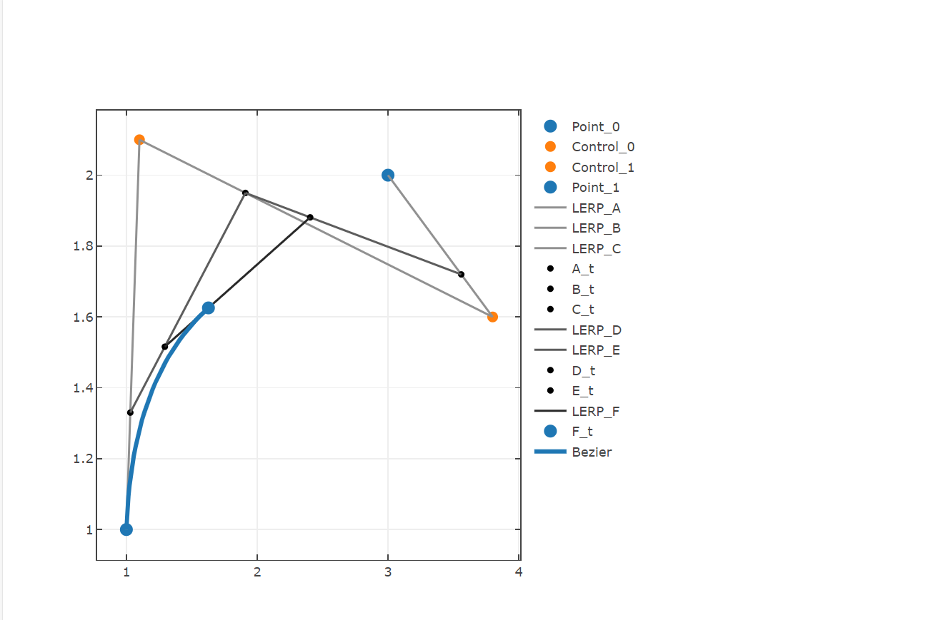
open FSharp.Stats
open FSharp.Stats.Interpolation
open Plotly.NET

let bezierInterpolation =
    let t = 0.3
    let p0 = vector [|3.;0.|] //point 0 that should be traversed
    let c0 = vector [|-1.5;8.|] //control point 0
    let c1 = vector [|1.5;9.|] //control point 1
    let c2 = vector [|6.5;-1.5|] //control point 2
    let c3 = vector [|13.5;4.|] //control point 3
    let p1 = vector [|10.;5.|] //point 1 that should be traversed
    let toPoint (v : Vector<float>) = v[0],v[1]
    let interpolate = Bezier.interpolate [|p0;c0;c1;c2;c3;p1|] >> toPoint

    [
        Chart.Point([p0.[0]],[p0.[1]],Name="Point_0",MarkerColor=Color.fromHex "#1f77b4") |> Chart.withMarkerStyle(Size=12)
        Chart.Point([c0.[0]],[c0.[1]],Name="Control_0",MarkerColor=Color.fromHex "#ff7f0e")|> Chart.withMarkerStyle(Size=10)
        Chart.Point([c1.[0]],[c1.[1]],Name="Control_1",MarkerColor=Color.fromHex "#ff7f0e")|> Chart.withMarkerStyle(Size=10)
        Chart.Point([c2.[0]],[c2.[1]],Name="Control_2",MarkerColor=Color.fromHex "#ff7f0e")|> Chart.withMarkerStyle(Size=10)
        Chart.Point([c3.[0]],[c3.[1]],Name="Control_3",MarkerColor=Color.fromHex "#ff7f0e")|> Chart.withMarkerStyle(Size=10)
        Chart.Point([p1.[0]],[p1.[1]],Name="Point_1",MarkerColor=Color.fromHex "#1f77b4") |> Chart.withMarkerStyle(Size=12)

        [0. .. 0.01 .. 1.] |> List.map interpolate |> Chart.Line |> Chart.withTraceInfo "Bezier" |> Chart.withLineStyle(Color=Color.fromHex "#1f77b4")
    ]
    |> Chart.combine
    |> Chart.withTemplate ChartTemplates.lightMirrored

(*** condition: ipynb ***)
#if IPYNB
bezierInterpolation
#endif // IPYNB

(***hide***)
bezierInterpolation |> GenericChart.toChartHTML
(***include-it-raw***)

(**

Bezier interpolation is not limited to 2D points, it can be also be used to interpolate vectors.

*)

let bezierInterpolation3d =
    let p0 = vector [|1.;1.;1.|] //point 0 that should be traversed
    let c0 = vector [|1.5;2.1;2.|] //control point 0
    let c1 = vector [|5.8;1.6;1.4|] //control point 1
    let p1 = vector [|3.;2.;0.|] //point 1 that should be traversed
    let to3Dpoint (v : Vector<float>) = v[0],v[1],v[2]
    let interpolate = Bezier.interpolate [|p0;c0;c1;p1|] >> to3Dpoint

    [
        Chart.Point3D([p0.[0]],[p0.[1]],[p0.[2]],Name="Point_0",MarkerColor=Color.fromHex "#1f77b4") |> Chart.withMarkerStyle(Size=12)
        Chart.Point3D([c0.[0]],[c0.[1]],[c0.[2]],Name="Control_0",MarkerColor=Color.fromHex "#ff7f0e")|> Chart.withMarkerStyle(Size=10)
        Chart.Point3D([c1.[0]],[c1.[1]],[c1.[2]],Name="Control_1",MarkerColor=Color.fromHex "#ff7f0e")|> Chart.withMarkerStyle(Size=10)
        Chart.Point3D([p1.[0]],[p1.[1]],[p1.[2]],Name="Point_1",MarkerColor=Color.fromHex "#1f77b4") |> Chart.withMarkerStyle(Size=12)

        [0. .. 0.01 .. 1.] |> List.map interpolate |> Chart.Line3D |> Chart.withTraceInfo "Bezier" |> Chart.withLineStyle(Color=Color.fromHex "#1f77b4",Width=10.)
    ]
    |> Chart.combine
    |> Chart.withTemplate ChartTemplates.lightMirrored

(*** condition: ipynb ***)
#if IPYNB
bezierInterpolation3d
#endif // IPYNB

(***hide***)
bezierInterpolation3d |> GenericChart.toChartHTML
(***include-it-raw***)



(**

## Chebyshev function approximation

Polynomials are great when it comes to slope/area determination or the investigation of signal properties.
When faced with an unknown (or complex) function it may be beneficial to approximate the data using polynomials, even if it does not correspond to the real model.

Polynomial regression can cause difficulties if the signal is flexible and the required polynomial degree is high. Floating point errors sometimes lead to vanishing coefficients and even though the
SSE should decrease, it does not and a strange, squiggly shape is generated. 
Polynomial interpolation can help to obtain a robust polynomial description of the data, but is prone to Runges phenomenon. 

In the next section, data is introduced that should be converted to a polynomial approximation.

*)


let xs = [|0. .. 0.2 .. 3.|]
let ys = [|5.;5.5;6.;6.1;4.;1.;0.7;0.3;0.5;0.9;5.;9.;9.;8.;6.5;5.;|]

let chebyChart =
    Chart.Line(xs,ys,Name="raw",ShowMarkers=true)
    |> Chart.withTemplate ChartTemplates.lightMirrored

(*** condition: ipynb ***)
#if IPYNB
chebyChart
#endif // IPYNB

(***hide***)
chebyChart |> GenericChart.toChartHTML
(***include-it-raw***)

(**
Let's fit a interpolating polynomial to the points:

*)

// calculates the coefficients of the interpolating polynomial
let coeffs = 
    Interpolation.Polynomial.interpolate (vector xs) (vector ys)

// determines the y value of a given x value with the interpolating coefficients
let interpolatingFunction x = 
    Interpolation.Polynomial.predict coeffs x

// plot the interpolated data
let interpolChart =
    let ys_interpol = 
        [|0. .. 0.01 .. 3.|] 
        |> Seq.map (fun x -> x,interpolatingFunction x)
    Chart.Line(ys_interpol,Name="interpol")
    |> Chart.withTemplate ChartTemplates.lightMirrored
    |> Chart.withXAxisStyle "xs"
    |> Chart.withYAxisStyle "ys"

let cbChart =
    [
    chebyChart
    interpolChart
    ]
    |> Chart.combine

(*** condition: ipynb ***)
#if IPYNB
cbChart
#endif // IPYNB

(***hide***)
cbChart |> GenericChart.toChartHTML
(***include-it-raw***)

(**
Because of Runges phenomenon the interpolating polynomial overshoots in the outer areas of the data. It would be detrimental if this function approximation is used to investigate signal properties.

To reduce this overfitting you can use x axis nodes that are spaced according to Chebyshev. Here, nodes are sparse in the center of the analysed function and are more dense in the outer areas. 

*)

// new x values are determined in the x axis range of the data. These should reduce overshooting behaviour.
// since the original data consisted of 16 points, 16 nodes are initialized
let xs_cheby = 
    Interpolation.Approximation.chebyshevNodes (Interval.CreateClosed<float>(0.,3.)) 16

// to get the corresponding y values to the xs_cheby a linear spline is generated that approximates the new y values
let ys_cheby =
    let ls = Interpolation.LinearSpline.interpolate xs ys
    xs_cheby |> Array.map (Interpolation.LinearSpline.predict ls)

// again polynomial interpolation coefficients are determined, but here with the x and y data that correspond to the chebyshev spacing
let coeffs_cheby = Interpolation.Polynomial.interpolate xs_cheby ys_cheby


// Note: the upper panel can be summarized by the follwing function:
Interpolation.Approximation.approxWithPolynomialFromValues(xData=xs,yData=ys,n=16,spacing=Approximation.Spacing.Chebyshev)

(**

Using the determined polynomial coefficients, the standard approach for fitting can be used to plot the signal together with the function approximation. Obviously the example data 
is difficult to approximate, but the chebyshev spacing of the x-nodes drastically reduces the overfitting in the outer areas of the signal.

*)

// function using the cheby_coefficients to get y values of given x value
let interpolating_cheby x = Interpolation.Polynomial.predict coeffs_cheby x

let interpolChart_cheby =
    let ys_interpol_cheby = 
        vector [|0. .. 0.01 .. 3.|] 
        |> Seq.map (fun x -> x,interpolating_cheby x)

    Chart.Line(ys_interpol_cheby,Name="interpol_cheby")
    |> Chart.withTemplate ChartTemplates.lightMirrored
    |> Chart.withXAxisStyle "xs"
    |> Chart.withYAxisStyle "ys"


let cbChart_cheby =
    [
    chebyChart
    interpolChart
    Chart.Line(xs_cheby,ys_cheby,ShowMarkers=true,Name="cheby_nodes") |> Chart.withTemplate ChartTemplates.lightMirrored|> Chart.withXAxisStyle "xs"|> Chart.withYAxisStyle "ys"
    interpolChart_cheby
    ]
    |> Chart.combine
    |> Chart.withTemplate ChartTemplates.lightMirrored
    |> Chart.withXAxisStyle "xs"
    |> Chart.withYAxisStyle "ys"


(*** condition: ipynb ***)
#if IPYNB
cbChart_cheby
#endif // IPYNB

(***hide***)
cbChart_cheby |> GenericChart.toChartHTML
(***include-it-raw***)


(**
If a non-polynomal function should be approximated as polynomial you can use `Interpolation.Approximation.approxWithPolynomial` with specifying the interval in which the function should be approximated.

## Further reading
- Amazing blog post regarding Runges phenomenon and chebyshev spacing https://www.mscroggs.co.uk/blog/57

*)