![]()
![]()

Prepared by Jakob Nybo Nissen, continued by Henry Webel
The first half of this Notebook contain a small introduction to numpy. You can also see a the YouTube video. If you feel comfortable using numpy, you can skip the introduction and go directly to the exercises (click here). If you would like a recap, keep reading on.
numpy is a Python package that provides a new type of object: The ndarray. This is an N-dimensional array, i.e. a "list" with any number of dimensions.
numpy is one of the most fundamental Python packages. Almost all of scientific Python uses numpy either directly, or indirectly through another package.
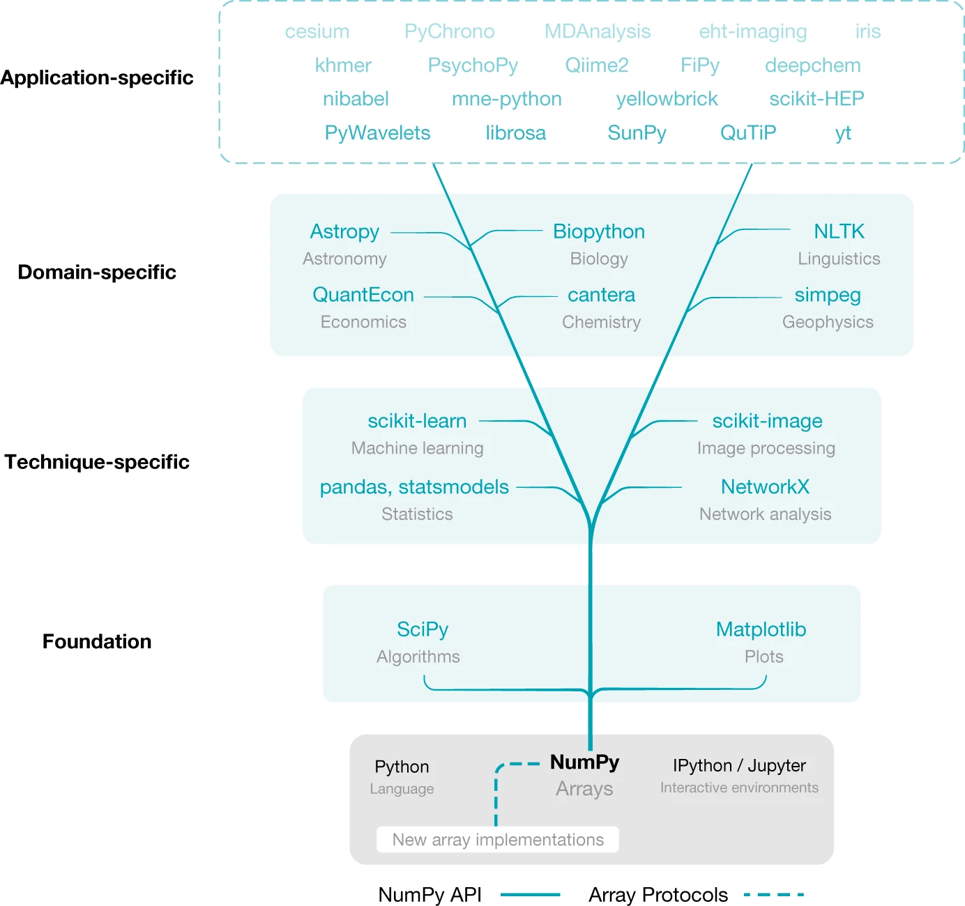
It may not be immediately clear why numpy's ndarrays are so useful that they are everywhere. Do ALL scientific software really need N-dimensional arrays? As you will learn in these exercises, even for 1-dimensional data that could be placed in lists, ndarrays are generally useful for their convenience and speed.
Harris, C. R., Millman, K. J., van der Walt, S. J., Gommers, R., Virtanen, P., Cournapeau, D., Wieser, E., Taylor, J., Berg, S., Smith, N. J., Kern, R., Picus, M., Hoyer, S., van Kerkwijk, M. H., Brett, M., Haldane, A., del Río, J. F., Wiebe, M., Peterson, P., … Oliphant, T. E. (2020). Array programming with NumPy. Nature, 585(7825), 357–362. https://doi.org/10.1038/s41586-020-2649-2
Today, first start with 1-dimensionalal ndarrays and use some statistical operations on them. Then, we will have a look at multidimensional arrays by using matrices, i.e. 2-dimensional ndarray's.
Let's get started right away and import numpy:
# We can import like this to rename numpy "np"
# and make the name shorter
import numpy as np
# # You can accces your drive files by connecting your drive storage
# from google.colab import drive
# drive.mount('/content/drive')We begin with a normal Python list of numbers. italicized text
values = [4, 9, 1, 0, 8, 3, 2, 2, 6, 5, 0]
values
[4, 9, 1, 0, 8, 3, 2, 2, 6, 5, 0]
We can create an ndarray out of this list using the constructor function numpy.array, which we pass some data:
array = np.array(values)
print(array)
print(type(array))
[4 9 1 0 8 3 2 2 6 5 0]
<class 'numpy.ndarray'>
You notice the ndarray looks a lot like a list. You can also construct ndarrays from a tuple.
There are many other ways to instantiate (i.e. create) ndarrays. Here are a few useful ones to create vector, i.e. 1d-ndarrays. You might need them later!
| function | Purpose | Example |
|---|---|---|
np.arange |
Makes an array with all the integers between two values | np.arange(2, 7) |
np.linspace |
Makes a specific-length array | np.linspace(2, 3, 10) |
np.zeros |
Makes an array of all zeros | np.zeros(5) |
np.ones |
Makes an array of all ones | np.ones(3) |
np.random.random |
Makes an array of random numbers | np.random.random(100) |
np.random.randn |
Makes an array of normally-distributed random numbers | np.random.randn(100) |
# Create a vector 10 zeros, default dtype is np.float64
print('np.zeros:', np.zeros(10, dtype=np.int64))

# Create an array of a range, similar to the range object
print('np.arange:', np.arange(3, 15, 2))

# Create vector of 10 floats from 3 to 15 having 9
# evenly spaced elements (linear spacing):
print('np.linspace:', np.linspace(3, 15, 9))

# Create a vector of random numbers in the interval [0.0, 1.0)
print('np.random.random:', np.random.random(5))

# Create 9 random integers from 7 to 18
print('np.random.randint:', np.random.randint(7, 19, size=9))
np.zeros: [0 0 0 0 0 0 0 0 0 0]
np.arange: [ 3 5 7 9 11 13]
np.linspace: [ 3. 4.5 6. 7.5 9. 10.5 12. 13.5 15. ]
np.random.random: [0.37876954 0.06446067 0.07600707 0.6318306 0.54057498]
np.random.randint: [18 15 8 13 15 16 10 7 11]
We can access and assign individual numbers in an ndarray like we do with list:
print(array)
print(array[2])
print(array[2:6])
array[3] = 10
print(array)
[4 9 1 0 8 3 2 2 6 5 0]
1
[1 0 8 3]
[ 4 9 1 10 8 3 2 2 6 5 0]
We can also loop over the ndarray, reverse it, and so on. The full list of methods you find in the docs of numpy.ndarray
There are two main limitations that ndarrays have compared to lists. We cannot use append or pop, or other operations that changes the array in-place:
array.append(3)---------------------------------------------------------------------------
AttributeError Traceback (most recent call last)
<ipython-input-52-e9cb6c9fca85> in <module>
----> 1 array.append(3)
AttributeError: 'numpy.ndarray' object has no attribute 'append'
We can however append several arrays together is slightly different way by using numpy.append(arr, values, axis=None) numpy.append
np.append([1, 2, 3], [1])np.append([1, 2, 3], [[4, 5, 6], [7, 8, 9]])- Define an array called
thingsthat 10 integers. The data is completely up to you. - Define an array of 20 random floats from 0 to 100
- Define an evenly spaced array of 20 random floats from 0 to 100
- Print out the second element in your array
things. - Append
[4, 5, 22]tothings - Remove
22fromthings(you need to find this one)
The second disadvantage is that an ndarray can only contain one kind of data at a time, i.e. float or int etc. The data type is given by the dtype field of the array:
array.dtypeThis array contains np.int64, a type representing 64-bit integers. If we try to add a float to the array, it will be converted to an np.int64, or raise an error if that is not possible.
# 1.7 can be "converted" by rounding down to 1
# (i.e) removing the fraction part, keeping the interger part 1
array[2] = 1.7
print(array)

# "hello" cannot be converted to an integer
array[2] = "hello" # "2" would work
[ 4 9 1 10 8 3 2 2 6 5 0]
---------------------------------------------------------------------------
ValueError Traceback (most recent call last)
<ipython-input-53-169bd88d1684> in <module>
5
6 # "hello" cannot be converted to an integer
----> 7 array[2] = "hello" # "2" would work
ValueError: invalid literal for int() with base 10: 'hello'
There is a type that allows mixing items of different type: object
array2 = array.astype('object')array2[2] = "hello"array2array([4, 9, 'hello', 10, 8, 3, 2, 2, 6, 5, 0], dtype=object)
There are many possible datatypes - you can read more about them on this link (click). However, we will only look at a few data types.
When you construct an ndarray, numpy will try to automatically detect the input data type:
array = np.array([1, 2, 3]) # again: constructor utility function np.array
print(array, array.dtype)

array = np.array([1.0, 2.0, 3])
print(array, array.dtype)
[1 2 3] int32
[1. 2. 3.] float64
Be careful when constructing ndarrays - for example if you try to construct an ndarray from a set object, which is not a list or a tuple, it simply create a 1-element ndarray containing the set as its only element, and the datatype will be object:
array = np.array({1,2,3})
print("array: ", array)
print("dtype: ", array.dtype)
array: {1, 2, 3}
dtype: object
You can also manually specify the data type you want. Notice here that it converts 2.5 to 2:
np.array([1.0, 2.5, 3.0], dtype=np.int64)array([1, 2, 3], dtype=int64)
And you can convert one numpy array to one with another dtype:
array = np.array([1, 2, 3])
array.astype(np.float64)
array([1., 2., 3.])
Conveniently, for many operations like +, -, *, /, ** and others apply to each element of an ndarray automatically. For example, if you write: array + 5, this will add 5 to every element in the array. This is termed vectorized operations:
array = np.array([4, 8, 1, 2, 9, 3, 7])
print(array)
print(array + 5)
print(array * 2)
print(array / 2)
print(array**2)
print(0.4 * array**2 + 1.5 * array - 0.9)
[4 8 1 2 9 3 7]
[ 9 13 6 7 14 8 12]
[ 8 16 2 4 18 6 14]
[2. 4. 0.5 1. 4.5 1.5 3.5]
[16 64 1 4 81 9 49]
[11.5 36.7 1. 3.7 45. 7.2 29.2]
Think about the difference of what the
+,-,*,/operators invoke in comparison tostrorlistbuilt-in types.
Because these vectorized operations actually execute code written in the programming language C, they are much, much faster than ordinary Python:
import random

# Create a vector of 1 million random floats in [0.0, 1.0):
python_list = [random.random() for i in range(1_000_000)]

# Convert the Python list to a Numpy vector
numpy_vector = np.array(python_list)%time results = [2*x + 3 for x in python_list] # List comprehension are optimizedWall time: 90 ms
%%time
collection_manipulated = []
for x in python_list:
    collection_manipulated.append(2*x + 3)
Wall time: 157 ms
# On Jacob's computer, this is >200x faster than Python
# In colab (with the lastest Python version?) this is still ~70x faster
# On my machine it is reduced to a 22x faster
%timeit results = 2*numpy_vector + 3
4.1 ms ± 109 µs per loop (mean ± std. dev. of 7 runs, 100 loops each)
Importantly, the comparison operators >, >=, <, <=, ==, != are also vectorized. Since these operators always return a bool (i.e. True or False), the result is an ndarray of data type bool. For example, we can check whether each element in array is greater than 3:
array = np.array([4, 8, 1, 2, 9, 3, 7])
mask_above_3 = array > 3
print(mask_above_3)
print(mask_above_3.dtype)
array[mask_above_3] # explanation: see next section
[ True True False False True False True]
bool
array([4, 8, 9, 7])
- Define an array of 100 random floats from 0 to 1000 and select those elements that are below 500
- In the same array, select those elements above 50 and below 300
If you are done, try to apply formulas to the whole data or try to change the
dtype
Logical indexing refers to indexing an ndarray using another ndarray of dtype bool. This selects every element of the ndarray paired with the value True: For example:
array = np.array([1, 4, 6, 5, 0, 2, 9, 10, 0, 2, 7, 5])
print('array:', array)
mask_nonzero = array != 0
print('nonzero:', mask_nonzero)

# Now get all elements that are not zero:
# Each element in array gets picked if nonzero is True
array[mask_nonzero]
array: [ 1 4 6 5 0 2 9 10 0 2 7 5]
nonzero: [ True True True True False True True True False True True True]
array([ 1, 4, 6, 5, 2, 9, 10, 2, 7, 5])
You can also assign to an ndarray using logical indexing. This will change all the numbers where the boolean array is True:
array[mask_nonzero] = 100
print(array)
[100 100 100 100 0 100 100 100 0 100 100 100]
To combine you can use the "bit-wise" operators & (logical and) and | (logical or), or one of the logical operations
In addition to the vectorized opertaions, the array object also have some methods (i.e. functions of the object type or class array) to conveniently perform operations on the arrays. Like vectorized operations, these methods are very fast. The full list of methods you find in the docs of numpy.array.
array = np.array([4, 8, 1, 2, 9, 3, 7])
print("Our array:", array)
print("Calculate sum:", array.sum())
print("Calculate mean:", array.mean())
print("Calculate variance:", array.var())
print("Calculate standard deviation:", array.std())
print("Calculate minimum/maximum:", array.min(), array.max())
Our array: [4 8 1 2 9 3 7]
Calculate sum: 34
Calculate mean: 4.857142857142857
Calculate variance: 8.408163265306122
Calculate standard deviation: 2.8996833043120627
Calculate minimum/maximum: 1 9
The methods performed on the ndarray can also be performed on different datastructures than arrays using numpy functions with idential names to the methods of an ndarray:
np.sum([4, 8, 1, 2, 9, 3, 7])34
Additional functions are not implemented as methods of ndarray, but can be found by typing np.FUNCITON_NAME such as:
np.log
np.sqrt
np.any
np.all,
and many, many more. In general, basic math operations, statistical operations and linear algebra is implemented in Numpy. Any other kind of number-crunching operation you might possibly need can be found in Scipy.
print(np.log(array)) # ln[1.38629436 2.07944154 0. 0.69314718 2.19722458 1.09861229
1.94591015]
The reason they are called ndarrays are that they are N-dimensional.
In the exercises, you can work on matrices, i.e. 2d-arrays.
First a little notation:
- A 1-dimensional array is a vector. A
2d-arrayis a matrix. An N-dimensional array is called a tensor or an array. - The number of dimensions of a tensor is its rank. So a matrix is a tensor of rank 2.
- In
numpy, the size of an array refers to the total number of elements. The shape of an array is a tuple with the length of the array in each of its dimensions. The length of an array is the length of the first dimension. - An axis is the same as a dimension.
Many ways of instantiating ndarrays have an optional keyword that allows us to specify its shape:
- list of list, etc
data = [[1, 5, 3, 9],
        [9, 4, 2, 4],
        [0, 6, 5, 1]]
data = np.array(data)
data
array([[1, 5, 3, 9],
[9, 4, 2, 4],
[0, 6, 5, 1]])
print("Shape:", data.shape)
print("Dimensions (Axes):", data.ndim)
Shape: (3, 4)
Dimensions (Axes): 2
data.reshape((4,-1))array([[1, 5, 3],
[9, 9, 4],
[2, 4, 0],
[6, 5, 1]])
- As we now have row and columns we can perform operations along the rows (
axis=0) or along the columns (row=1). What is the mean along the rows? What along the columns?
see the methods section for further methods
print(data)
data.sum() # default along all axis
[[1 5 3 9]
[9 4 2 4]
[0 6 5 1]]
49
data.sum(axis=0)array([10, 15, 10, 14])
data.sum(axis=1)array([18, 19, 12])
- sometimes needed for broadcasting (next sections)
- You might need this if you later move to machine learning and start using sklearn
data[:,:, np.newaxis].shape
np.expand_dims(data, axis=-1).shape
(3, 4, 1)
Removing a trailing axis is done using squeeze
data = np.expand_dims(data, axis=-1)
data = data.squeeze()
data.shape
(3, 4)
Broadcasting is a technique automatically matching arrays of different shape - if they are compatible. Read the numpy guide on broadcasting (which is the default behaviour in many array libraries)
data * 5array([[ 5, 25, 15, 45],
[45, 20, 10, 20],
[ 0, 30, 25, 5]])
data / data.sum(axis=1)[:, np.newaxis]array([[0.05555556, 0.27777778, 0.16666667, 0.5 ],
[0.47368421, 0.21052632, 0.10526316, 0.21052632],
[0. , 0.5 , 0.41666667, 0.08333333]])
In all of these exercises, do not loop over the ndarrays you create. All exercises can be solved using only vectorized operations on your arrays.
You want to plot the mathematical function
For the numbers in xs with lots of numbers between 0 and 20, and a vector ys with xs. A vector is a 1d-ndarray.
To get a hang of vectorized operations, solve the problem without using any loops:
Hint: You can use a comparison operator to get an array of dtype
bool. To get the number of elements that areTrue, you can exploit the fact thatTruebehaves similar to the number 1, andFalsesimilar to the number 0.
Load in the data depths.csv. As you can see loading the first line below, there are 11 columns, with columns 2-11 representing a sample from a human gut microbiome. Each row represents a genome of a micro-organism, a so-called "operational taxonomic unit at 97% sequence identity" (OTU_97). The first row gives the name of the genome. The values in the matrix represents the relative abundance (or depth) of that micro-organism in that sample, i.e. how much of the micro-organism there is.
# If you have a local copy of the repository, this is the path to the file depths.csv
from pathlib import Path
filepath = Path('../data/depths.csv')
# Download in colab
# You can use Bash commands by prepending them with: !
if not filepath.exists():
!mkdir -p data
!wget https://raw.githubusercontent.com/pythontsunami/teaching/intro/data/depths.csv -P data
filepath = Path('data/depths.csv')with open(filepath) as file:
for i, line in enumerate(file):
print(line)
if i > 5:
break#genome,sample_6,sample_7,sample_8,sample_13,sample_14,sample_15,sample_16,sample_17,sample_18,sample_19
OTU_97.21068.0,1.4179,0.3905,0.0000,0.0000,0.0000,0.0000,1.6318,0.3905,0.0000,0.0000
OTU_97.360.0,0.3871,0.0000,0.0000,0.0000,0.0000,0.0000,0.3871,0.0000,0.0000,0.0000
OTU_97.44228.0,7.5783,87.6600,13.1089,28.6166,25.1856,10.2906,37.3140,104.9891,13.1089,49.1341
OTU_97.38344.1,1.9753,0.0000,0.0000,0.0000,0.0000,0.0000,2.2735,0.0000,8.8969,0.0000
OTU_97.28595.0,7.5782,2.0872,7.8652,0.0000,0.0000,0.0000,9.8654,2.0872,7.8652,0.0000
OTU_97.17212.1,0.9032,0.0000,0.0000,0.0000,0.3752,0.0000,0.9032,0.0000,0.0000,0.0000
Load in the matrix in some data structure of your choice, but make sure the numbers in each row is an ndarray.
Find the OTU "OTU_97.41189.0". What is the mean and standard deviations of the depths across the 10 samples of this OTU?
After discarding all OTUs present in fewer than 4 samples, sort the OTUs, do the following:
- Calculate the mean depth across samples for each remaining OTU.
- Normalize the remaining OTUs such that each row sum to 0 and have a standard deviation of 1 (so-called z-score normalization)
- Print the remaining OTUs to a new file in descending order by their mean depth, with a 12th column giving the mean depth, and columns 1-11 being the normalized depth. Make sure that your file looks like the input file (except with the 12th column)
----------------------------------------------------------------------------------------------------------------------------------
----------------------------------------------------------------------------------------------------------------------------------
Only do it if you have extra time.
Create a function that loads a FASTA file into a dict where each key is the FASTA header and the value is an ndarray corresponding to the sequence. Remember that you need to instantiate ndarray from a list, not a string. Test it using the Yersinia pestis fasta file. You can verify that your ndarray has the correct length by checking the .size attribute:
array.size
Make your function verify that there are only 'A', 'C', 'G', 'T' and 'N' in the sequence. Convert lowercase letters to uppercase letters.
Create a function that calculates GC content of your ndarray representing a DNA sequence - ignore Ns. Remember to still use vectorized operations.
Use the Jupyter %timeit functionality to compare the time spent in your vectorized GC-content function with the GC-content function you created in exercise 2 last monday. See the use of %timeit in this Notebook for an example.